Pipeline overview
The FLOYDS IRAF-based pipeline is unsupported for data taken at the COJ spectrograph, and will be completely deprecated as of May 1st 2026. From then on, BANZAI-Floyds is the only LCO-supported data pipeline for Floyds.
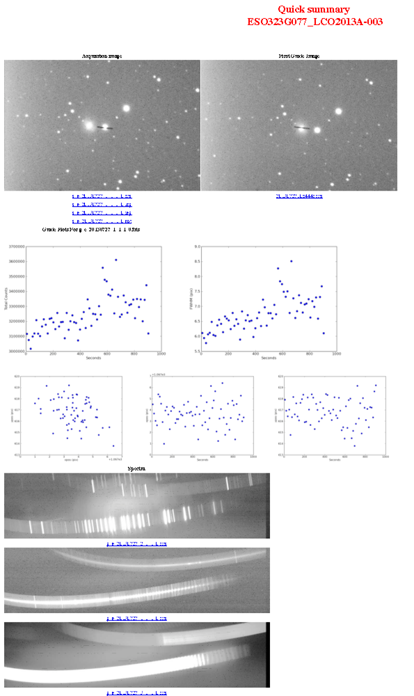
The FLOYDS pipeline runs at LCO headquarters after the observing nights at FTN (Hawaii) and FTS (Australia) end. The pipeline produces a tar file that includes the raw observations, an automatically extracted spectrum, and the guider images that can be used for quality control. Intermediate data products are also provided so that the user can, for example, re-extract the spectrum (from the wavelength-calibrated, flux-calibrated, and rectified 2-D images).
It is also possible to install and run the FLOYDS pipeline interactively, but this is not described here.
Analysis on the 2-D Frames
The pipeline initially performs the following operations on the science, arc, and flat field frames:
- Splitting orders: In the raw exposures, the first ("red") and second ("blue") order are in the same image, so the first step is to split the orders into separate files. From here on, the red and blue orders are analyzed separately and only combined at the end.
- Rectification: The spectra are initially curved, so the 2-D frames are resampled to straighten (rectify) the trace. The transformation function is approximated using Legendre polynomials; the coefficients for FLOYDS at FTN and FTS were determined during commissioning. Tests indicated that the spectrographs are stable enough to use a fixed transformation function, rather than computing the transformation from each data set. The fixed function insures that the rectification will succeed even for data with a low signal-to-noise ratio.
- Trimming: The frame is trimmed to exclude regions of the image with no signal.
- Cosmic Ray Cleaning : Cosmic rays are removed from the 2-D images using the lacosmic Laplacian cosmic ray rejection algorithm from van Dokkum (2001). Specifically, we use a Python implementation, cosmics.py, that we have modified to remove its dependency on the scipy package.
- Wavelength Rectification: At this point, the trace of a source will be roughly horizontal, but the arc/sky lines are still slanted. We now resample the 2-D frame such that each column corresponds to a single wavelength (i.e. the arc/sky lines are vertical). As with the trace rectification, we use a fixed transformation function with Legendre polynomials. This has the added benefit of producing a rough wavelength calibration. The wavelength calibration can later be refined using the arc spectra (if available) or sky lines.
- Flat-field Correction: We divide out a normalized flat field image. Flat fields are normalized using the pyraf task apflatten, which uses a fitted low order polynomial surface to normalize the flat frames. This task gives a better result that the IRAF task response when significant fringing is present, as is the case for FLOYDS. If the flat field frames were taken in the same observation block as the science spectrum, the flat-field correction can reduce the effects of fringing. Because fringing is prevelant in the red arm of FLOYDS, we attempt to scale the flat to optimally remove the fringes, but we are investigating better solutions. Currently only the red arm is flat fielded; an internal dichroic is used on the blue arm. Both the flat-field corrected and uncorrected frames are included in the data product.
- Wavelength Solution Refinement: Using the sky lines and telluric absorption features, we refine the initial wavelength solution.
- Flux calibration: We flux calibrate the 2-D science frame using the sensitivity function derived from flux standard star observations taken during commissioning. Like the rectification transformations, the sensitivity function is fixed for all data sets. The flux calibrated spectra are saved in units of 10-20 ergs / s / cm2 / Å. We provide flux calibrated 2-D frames both with and without the flat field correction.
- Trace Extraction: When we have the 2-D flux calibrated frames, we run a preliminary 1-D extraction using the automatic trace detection features from the IRAF task apall on both the red and blue arms.
- Merging Red and Blue: Finally, we merge the red and blue 1-D extracted traces to create the final 1-D reduced spectrum.
While the preliminary extracted 1-D spectrum may be useful to check the data quality, we consider the 2-D wavelength and flux calibrated image (shown below) the best starting point for users. We encourage users to manually perform the final stages:
- Extraction: Depending on the science goals for a project, differing extraction parameters may be necessary. Some parameters that we expect would vary from one science case to another are the size, location, and number of the extraction apertures and how the background is subtracted. The user may do this using the IRAF task apall.
- Wavelength Solution Refinement: The automatic pipeline does not use arc lamp observations that were taken with the science exposure. The fixed wavelength calibration should be accurate to 1-2 Å. The user is encouraged to refine the wavelength solution using arc lamp observations taken with their science observation. If arc lamp observations were taken with the science spectrum, we provide the 2-D, rectified, arc lamp frames. These can be applied to improve the wavelength solution using, for example, the IRAF task identify. Wavelength calibration accurate to a few tenths of an Angstrom should be possible by applying arc lamp observations taken with the science exposure.
- Flux Calibration Refinement: Standard star observations are publicly available through the archive. We encourage users to recalibrate the flux of spectra using standard star observations that were taken as close in time to the science spectrum as possible.
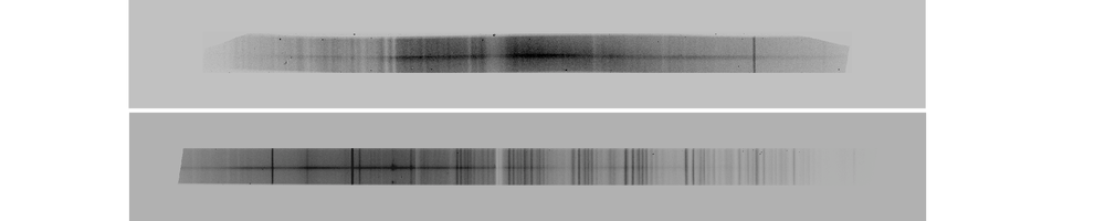
Fig. 1 Example 2-D rectified, flux calibrated products from the FLOYDS Pipeline.
FLOYDS Data Products
The processed FLOYDS data can be retrieved from the LCO science archive. Users can search for data by Proposal ID, date, telescope site, object name, etc. All of the data products for each observation are packaged into a single tar file. The naming convention for the tar file is {Proposal ID}_{Block ID}_{Telescope}_{Day-Obs}_{MJD Reduced}.tar.gz. The Day-Obs corresponds to the local observing night on which the spectrum was taken (this may differ by one day from the UTC date of observation). The MJD Reduced is the Modified Julian Date when the reduction was performed. Because the reduction is done after the local end of the night, the MJD Reduced may be different from the Day-Obs. The Block ID is an internal identifier that is used to associate calibration frames (e.g. arcs and flats) that are taken as part of the same request as the science spectrum.
For example:
LCO2016B-011_0001019682_fts_20170331_57844.tar.gz
The raw data files follow the standard LCO naming convention (e.g. for images). The individual processed data products inside the tar file are named according to {File Type}{Object Name}_{Telescope}_{Day-Obs}_{red/blue}_{Slit Width}_{MJD Reduced}_{Spectrum Number}_{Flux calibrated}.fits. For the file type, the prefix “tt” indicates that the frame has been rectified in both the spatial and wavelength directions, while “n” indicates that the frame has been flat field corrected. The spectrum number corresponds to the exposure number in the block: e.g. for a request that had 2x1800s science spectra, the second exposure would have exposure number = 2. The extension “2df” indicates a flux calibrated spectrum. The final extension "ex" indicates a 1-D extraction of the brightest trace in the frame. The sensitivity functions that were used have a prefix of "sens".
An example set of data products is below: