Materials List
Per student:
- A computer with Internet connection
- Hubble Diagram Student Spreadsheet (xls)
- Hubble Diagram Instruction Sheet (PDF)
During this activity students will use real supernova spectra to create a famous Hubble Diagram and calculate the age of the Universe.
Per student:
Measuring distances in space is a daunting task. One method is to use an object with a known absolute magnitude (M); we call these Standard Candles. Type Ia supernovae are standard candles.
There are two classes of supernovae, Type I and Type II. For this activity we will be using Type Ia supernovae only. Type Ia supernovae are very important in astronomy as they offer the most reliable sources for measuring cosmic distances up to and beyond 1000 mega parsecs (Mpc). A parsec (pc) is a unit of length used to measure the distances to objects in space. One parsec is equal to 3.08567758 × 10¹⁶ metres.
Type Ia supernova are thought to form when a white dwarf star accretes enough mass from a companion star to exceed the upper limit of 1.44 solar masses, which causes the star to explode as a supernova.
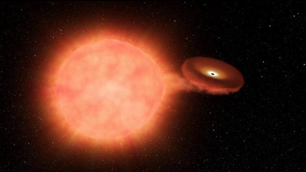
Image credit: NASA/JPL-Caltech
This model implies that all Type Ia supernovae start with essentially the same mass and therefore the energy output from the resulting supernova should always be the same. Of course, it is not quite that simple, but all Type Ia supernova do seem to have similar light curves and can therefore be related to the same common template. There is an average maximum absolute magnitude that these supernovae can reach in the visible wavelength band B. The peak brightness is: -19.6 mag.
If we also know the apparent magnitude for a Type Ia supernova, we can use the distance modulus to calculate its distance from earth. The distance modulus is the difference between the apparent magnitude (m) and the absolute magnitude (M) of an astronomical object. It can be used to provide the distance (d) in parsecs. Once m is known, the distance modulus function can be used to calculate the distance to the supernova in parsecs (pc):
d=10((m - M + 5)/5) pc
To create a Hubble Diagram, the redshift and velocity of your object is needed, as well as the distance. To find the redshift of an object astronomers use spectroscopy. Spectroscopy is a branch of science that is concerned with the investigation and measurement of the spectrum of light produced when matter interacts with electromagnetic radiation. In astronomy, spectroscopy is a very useful tool because telescopes can easily measure the spectra of far away objects, such as stars and galaxies.
We measure the spectra of luminous objects by attaching a special instrument to a telescope, known as a spectrograph. Within the spectrograph, light is passed through a series of prisms and mirrors in order to split the light into its different component wavelengths (its spectrum). The intensity of those different wavelength components is then measured to create a spectrum. The spectrum can then be investigated in detail to discover useful information about the target such as chemical composition, Doppler shift and velocity.
The Doppler Effect, such as redshift, occurs due to an apparent shift in the wavelength and frequency of a wave due to relative motion between the source and the observer. For example, we experience the Doppler Effect when an ambulance drives past with its sirens on:

Illustrating demonstrating the Doppler effect, with the shortest wavelength on the left and longer wavelengths on the right.
The same effect is observed with light, when an object is moving towards or away from observers located on the Earth. We can detect this motion in the spectrum of the star.
If the star is moving away from the Earth, the light waves are stretched out and the whole spectra experiences a shift towards the red end of the spectrum – a red shift. If the star is moving towards the Earth, the light waves are bunched up and the spectra experiences a shift towards the blue end of the spectrum – a blue shift.
We can measure comparing an observed wavelength to a rest wavelength. For example, the rest wavelength for Hα (when there is no Doppler Effect) is 6563Å, if it is redshifted the observed wavelength will be longer. If both the observed and rest wavelengths are known, these can be used to calculate the object’s redshift, where z = redshift:
z = (observed wavelength/rest wavelength) – 1
The idea that we live in an expanding Universe was one of the most unexpected and important discoveries of the 20th century. Until then, everyone, including astronomers, had assumed that the Universe was a stable, unchanging stage on which astronomical events played themselves out. But then, in the early 1900s scientists made several discoveries that defied easy explanation. These discoveries came together in the mind of an astronomer named Edwin Hubble, who explained all of them in 1929 with the expanding universe theory.
The discovery of the expanding universe was, like more discoveries, a combined effort. In the early 1900s an American astronomer called Vesto Slipher studied the spectra of a number of “fuzzy objects” believed to be nebula (we now know many of them were separate galaxies). He noticed that many of them were redshifted, which meant they were moving away from us. Some of them were moving away from us at amazing speeds – for example the object we now know of as the Sombrero Galaxy was moving away from us at speeds of 4 million km per hour.

Portrait of Edwin Hubble
While Slipher made this discovery, in another part of the world Edwin Hubble was using the world's biggest telescope (at the time) to measure the distance to astronomical object using creative new methods. Hubble then compared his measurements of distance, to Slipher’s measurements of redshift and plotted the results – this plot is now known as the Hubble Diagram.
The Hubble diagram demonstrated that a galaxy’s redshift increased linearly with its distance from Earth. The farther away a galaxy is, the faster it moves away from us.
The simplest explanation for Hubble’s observation was that the entire universe is expanding, just as Einstein's equations predicted it should. If the universe is expanding, then at some time in the past, it must have started from a single point - an idea known as the Big Bang. Hubble's discovery, and the later development of the big bang theory, changed astronomy forever.
In this activity students will follow the steps on the student handout to plot the famous Hubble Diagram to demonstrate the expanding Universe, beginning by determining the redshift for 10 Type Ia supernovae, from which they will derive the radial velocity for each supernova. They will then calculate the distance to each supernova and use the two values to plot the famous Hubble Diagram.
Once they have plotted the Hubble Diagram, your students will study their results and hopefully come to the conclusions that Hubble reached, now known as Hubble’s Law. Hubble's law is the name for the observation in physical cosmology that: (1) objects observed in deep space (extragalactic space which is more than 10 Mpc) are found to have a Doppler shift that can be used to calculate their relative velocity away from the Earth; and (2) that the velocity, of various objects receding from the Earth, is approximately proportional to their distance from the Earth. This is normally interpreted as a direct observation of the expansion of the Universe.
The expansion of the Universe was first proposed by Georges Lemaître in 1927, he also suggested an estimated value of the rate of expansion, now called the Hubble Constant. Hubble also calculated a value for the Hubble Constant just two years later, he put it at around 500 km/s/Mpc. We now know this was incorrect. Based on the latest results, the Hubble Constant is believe to be 73 km/s/Mpc.
In this activity your students will also calculate the Hubble Constant based on their own Hubble Diagram.
In this activity you will begin by selecting ten different Type 1a supernovae. Using their spectra, you will calculate their redshift before using your results to derive the radial velocity for each supernova. Next, you will calculate the distance to each of your objects before using these two values to plot the famous Hubble Diagram.
This website is an archive containing spectra for a number of different types of astronomical object collected by a range of instruments. For this activity we will be using spectra for Type Ia supernovae collected by the LCO FLOYDS spectrograph and the STIS spectrograph aboard the Hubble Space Telescope.
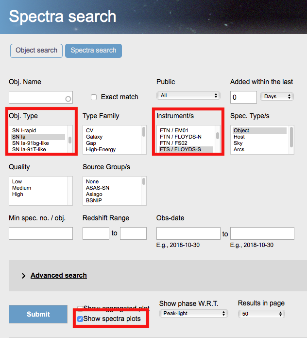
Note: Be careful to ensure that you have ten different supernova spectra and have not duplicated any, as there are multiple spectra for some supernovae.

To understand how the redshift was calculated, continue to section II. Calculating Redshift, otherwise jump to section III. Calculating Radial Velocity
You will see two values for the chosen wavelength (WL) below the graph: observed and rest. These values show us how the supernova is moving relative to us. The wavelength is shown in a unit called Ångström (Å). Make a note of the observed wavelength and rest wavelength values on your worksheet.
Take some time to explore these elements and find out which are present in each object, the more defined the feature, the heavier the presence of these elements. Which element is most abundant in this supernova? Note down your answer in the ‘Element’ column on your worksheet on the appropriate row.
z = (observed wavelength/rest wavelength) – 1
Question: Refering back to the redshift provided by WISeREP, is it that same as your redshift for each of your supernova?
Using the redshift values you have calculated, we are now able to derive the radial velocity for each supernova using the simple equation:
radial velocity = redshift × speed of light
An example, if a supernova has a redshift of 0.025, then the radial velocity is given by
radial velocity = 0.025 × 300000 = 7500 km/s
Note: This equation only works for redshift smaller than z = 1.0.
Discussion question: You may have noticed that all your redshift figures are positive. What would it mean if your redshift were negative?
The final piece of information we need to plot our Hubble Diagram is the distance to each supernovae. Measuring distances in space is a daunting task. One method of measuring distances is to use an object with a known absolute magnitude (M), we call these Standard Candles. Type Ia supernovae are standard candles.
Type Ia supernovae happen when a white dwarf star reaches 1.4 solar masses causing a nuclear chain reaction to occur that causes the star to explode. This chain reaction always happens in the same way and at the same mass, which means the brightness of Type Ia supernovae is always the same, a peak light output approximately equivalent to an absolute blue sensitive magnitude of -19.6.
Apparent magnitude (m) is how bright an object appears in the sky, this is a function of both its actual light output, known as it’s absolute magnitude (M), and it’s distance from the observer. If we have values for the former two, we are able to calculate the latter.
Once m is known, the distance modulus function can be used to calculate the distance to the Type Ia supernova in parsecs (pc):
m - M = 5 log d – 5
Rearranged:
d = 10((m - M + 5)/5) pc
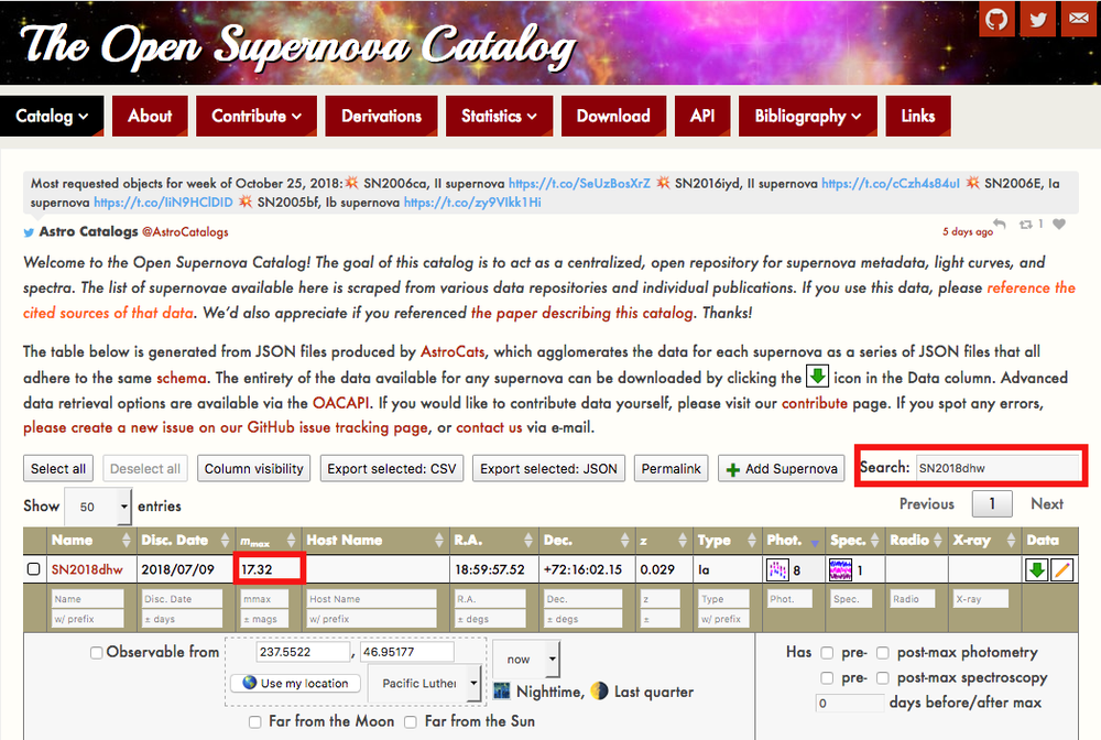
If the B-band magnitude for your supernovae has not been provided, go to the Open Supernova Catalog homepage and enter your object name into the Search field.
There is a column in the table called B-band max (mag) this shows the maximum apparent magnitude (m) for each supernovae.
Note: If you still cannot locate the B-band maximum magnitude for your chosen supernova, return to section I. Finding Redshift and select new supernovae for which you have the B-band magnitude.
Alternatively, enter m and M for your supernovae where indicated on the 'Calculations' tab of your worksheet and the distance will be automatically calculated in Mpc.
This line allows you to make an estimate of the Hubble constant. The Hubble constant is the gradient of this line.
The Hubble constant (H0) is one of the most important numbers in cosmology because it can be used to estimate the size and age of the Universe. The Hubble constant indicates the rate at which the Universe is currently expanding, so although it is called a ‘constant’ it changes with time.
The Hubble constant is give by:
H0 = v/d
Where v is the radial velocity, d is the distance and the 0 denotes that the number derived is the Hubble constant at the present time. The value for the Hubble constant is given in kilometres per second per mega parsec (Mpc).
You’ve now successfully determined the rate of the expansion of the Universe!
Ask the students to answer the following questions.
Now that you have a value for the Hubble constant, one simple thing you can do to wrap up the activity is estimate the age of the Universe. This can be done by finding the inverse of the value of Ho .
1. If the Universe has been expanding at a constant speed since its beginning, the Universe's age would simply be 1/Ho
Assuming this is true, calculate the age of the Universe using your value for the Hubble Constant.
2. Next, multiply you answer by 3.09 x 10¹⁹ km/Mpc to cancel the distance units. You now have the age of the Universe in seconds!
3. Divide this number by the number of seconds in a year: 3.16 x 10⁷ sec/yr
4. Now you have worked out the age of the Universe in years using real observational data!

Extended (60+ mins)