Exposure Time Estimating

This guide will give you a background to how astronomical CCDs and cameras work, how to choose an appropriate signal to noise ratio, and finally how to estimate a reasonable exposure time for your target.

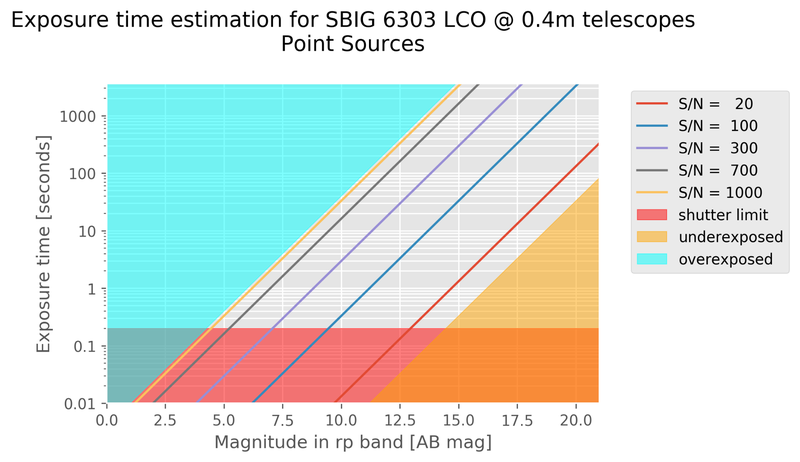
If you just want to look up an appropriate exposure time, please use the graph below.

1. Dynamical Range and Saturation Limit of SBIG camera

There are two factors governing the useful output range of a detector:

1. The charge that a pixel can hold.
2. The dynamical range of the analog to digital converter (ADC) in the CCD controller.

Let's have a look how these two effects work.

The full well

As a photon is absorbed in a CCD pixel, it is converted into an electron (photo effect). The pixel itself is usually defined by an isolating layer in one direction (usually the x, serial register direction), and by an electrical field in the other direction (usually y, parallel register direction). During the readout process, the electric field that defines a pixel is clocked, and the charge is moved towards an output capacitor capacitor where the charge signal is converted into a voltage (capacity = charge per voltage).

During an exposure, charge accumulates in a pixel. At some point, the electric field that defines a pixel cannot hold the charge in place, and when the charge is too high (i.e., the image overexposed), it will overflow (“blooming”) into neighbouring pixels. The amount of charge where this effect starts to become relevant is called “full well”, and is usually measured in the unit of number of electrons. For astronomical CCDs, the full well is of the order of fifty to a few hundred thousand electrons, and is a real physical limitation of a detector.

The full well defines how much light a pixel can sense before it saturates, i..e, overexposes.

The ADC dynamic range

The output voltage from the CCD detector is proportional to the charge that was in a pixel. This output voltage is usually amplified, and then fed into a analog to digital converter (ADC): The light received in a pixel will be converted into a computer-readable number. There are design choices to be made in a CCD controller when selecting the electrical parts:

1. In general it is desirable that the the range of voltages from the CCD (e.g., 0 Volt output dark, 0.5 Volt when the full well capacity has been reached) is amplified to match the input range of the ADC part (e.g., 0 Volts to 5 Volts). Some CCD controllers allow to change this amplification to adopt to a range of CCDs or readout modes.
2. Typically, ADC parts used in CCD controllers use 16 bits to represent the output number (0 to 65536). There are some controllers that can use 32 bit outputs, some use fewer bits (e.g., 14).

Ideally one would match the CCD output and amplification such that when there is no light, the ADC reports a small number, and the maximum number (e.g., for 16 bit, 65536) when the full well of a pixel is reached. It is possible, however, that a system was designed such that the dynamical range of the ADC is reached well before the full well was reached and vice versa - there are good reasons to do this, depending on the actual application.

The Gain

As we have seen above, the number output of an ADC is proportional to the number of electrons that were in a CCD's pixel, which was proportional to the number of photons detected. So:

Pixel Value [ADU] ∝ number electrons [e-]

The factor in this relation is called gain and has the unit of electrons per ADU (ADU = Analog Digital Unit) or e- / ADU.

Let's say that the full well capacity of a pixel in our CCD was 200000 electrons. One would design the CCD controller such that these 200000 electrons could be mapped into a range of a 16 bit number. That would lead to a gain of 200000 e- / 65536  ADU ~ 3 e- / ADU . Note that a 16 bit number has not enough resolution to properly sample the range of 200000 electrons!

Full well and gain for the 0.4m SBIG cameras

As of June 1st 2018, the SBIG cameras at LCO will operate in an unbinned mode. In that configuration the full well per pixel is of the order of 100,000 e-, and the gain is approximately 1.6 e-/ ADU. The best known value of full well and gain are captured in an image header in the keywords, for example:

GAIN = 1.6000000 / [electrons/count] Pixel gain
SATURATE= 124000.0000000 / [ADU] Saturation level
MAXLIN = 102000.0000000 / [ADU] Non-linearity level

Full well and gain in Calibrated data

All LCO imaging data are processed with the BANZAI calibration pipeline. As part of the process, the pipeline will multiply the images by their gain, and then set the GAIN header keyword to 1 e-/ADU. In the example above, for raw images one will find a GAIN of 1.6 e-/ADU and a saturation limit (SATURATE) of 64000 ADU.  After processing, the counts in the images will be multiplied with the gain, the header keywords are GAIN=1 e-/ADU and SATURATE=102400 ADU. The maximum capacity of the detector pixels in units of electrons stays the same, it is just represented on a different scale in the processed image files.

2. How to choose a Signal to Noise

The relative error of a measurement is called Signal to Noise ratio, S/N. For the signal from a star, the noise is the square root of the signal (shot noise), i.e., the Signal to noise ratio would be Signal / Sqrt(Signal). In the following we will ignore other noise sources, such as detector noise, or systematic errors such as flat field errors.

Let's get a feeling for what S/N means:

Note that if an photometric error of 0.1% is desired, one needs to collect at least 1,000,000 photons just to overcome the shot noise. We learned that the full well of a pixel is of order of 100,000 electrons. This means, one cannot measure the flux of a star with a CCD at a high fidelity if the light was collected in a single pixel. One would either have to combine the result of several exposures, expose the star onto several pixels on the detector, or a combination thereof.

For most ground-based imagers, the turbulence of the atmosphere smears out the image of a star (called “seeing”).  A detector is usually selected such that the width of the seeing disk is a few pixels in size. At the LCO 0.4m telescopes, the typical full width, half maximum size of the star images is of order of 4 to 5 pixels.  

3. Desirable Exposure time per target.

We have seen that the saturation limit of a pixel, the full well, limits how much light we can collect from an object in one single exposure. On the other hand, one wants to collect as much light as possible to limit the uncertainty of a flux measurement. A third consideration is that telescope time is precious, and one should not observe longer than required to achieve a scientific goal.

Mixing this together, the first question an observer should ask: At what accuracy do I need to measure the flux of my target? Once that questions is answered, one selects an appropriate exposure time. To aid this process, we have created the graph below, where we show for a range of stellar magnitudes in the r' band the Signal to Noise that can be achieved in a given exposure time.

The red shaded region indicates the minimum achievable exposure time with the cameras - we can't get any faster with the camera. The lower right shaded region indicates the zone of underexposed images. The upper left shaded region shows where exposures would saturate for an object.